THE COMPUTER AND THE BRAIN. JOHN VON NEUMANN.1958. A Puke (TM) Audiobook
THE COMPUTER AND THE BRAIN.
JOHN VON NEUMANN.
First edition 1958.
For historical interest.
INTRODUCTION.
Since I am neither a neurologist nor a psychiatrist, but a mathematician, the work that follows requires some explanation and justification. It is an approach toward the understanding of the nervous system from the mathematician’s point of view. However, this statement must immediately be qualified in both of its essential parts.
First, it is an overstatement to describe what I am attempting here as an “approach toward the understanding”; it is merely a somewhat systematized set of speculations as to how such an approach ought to be made. That is, I am trying to guess which of the, mathematically guided, lines of attack seem, from the hazy distance in which we see most of them, a priori promising, and which ones have the opposite appearance. I will also offer some rationalizations of these guesses.
Second, the “mathematician’s point of view,” as I would like to have it understood in this context, carries a distribution of emphases that differs from the usual one: apart from the stress on the general mathematical techniques, the logical and the statistical aspects will be in the foreground. Furthermore, logics and statistics should be primarily, although not exclusively, viewed as the basic tools of “information theory.” Also, that body of experience which has grown up around the planning, evaluating, and coding of complicated logical and mathematical automata will be the focus of much of this information theory. The most typical, but not the only, such automata are, of course, the large electronic computing machines.
Let me note, in passing, that it would be very satisfactory if one could talk about a “theory” of such automata. Regrettably, what at this moment exists, and to what I must appeal, can as yet be described only as an imperfectly articulated and hardly formalized “body of experience.”
Lastly, my main aim is actually to bring out a rather different aspect of the matter. I suspect that a deeper mathematical study of the nervous system, “mathematical” in the sense outlined above, will affect our understanding of the aspects of mathematics itself that are involved. In fact, it may alter the way in which we look on mathematics and logics proper. I will try to explain my reasons for this belief later.
PART One. THE COMPUTER.
I begin by discussing some of the principles underlying the systematics and the practice of computing machines.
Existing computing machines fall into two broad classes: “analog” and “digital.” This subdivision arises according to the way in which the numbers, on which the machine operates, are represented in it.
The Analog Procedure.
In an analog machine each number is represented by a suitable physical quantity, whose values, measured in some pre-assigned unit, is equal to the number in question. This quantity may be the angle by which a certain disk has rotated, or the strength of a certain current, or the amount of a certain (relative) voltage, etc. To enable the machine to compute, meaning to operate on these numbers according to a predetermined plan, it is necessary to provide organs, or components, that can perform on these representative quantities the basic operations of mathematics.
The Conventional Basic Operations.
These basic operations are usually understood to be the “four species of arithmetic”:
Addition (the operation x plus y), subtraction (x minus y), multiplication (x times y), division (x dived by y).
Thus it is obviously not difficult to add or to subtract two currents (by merging them in parallel or in antiparallel directions). Multiplication (of two currents) is more difficult, but there exist various kinds of electrical componentry which will perform this operation. The same is true for division, of one current by another. For multiplication as well as for division, but not for addition and subtraction, of course the unit in which the current is measured is relevant.
Unusual Basic Operations.
A rather remarkable attribute of some analog machines, on which I will have to comment a good deal further, is this. Occasionally the machine is built around other “basic” operations than the four species of arithmetic mentioned above. Thus the classical “differential analyzer,” which expresses numbers by the angles by which certain disks have rotated, proceeds as follows. Instead of addition, x plus y, and subtraction, x minus y, the operations (x plus or minus y) divided by two are offered, because a readily available, simple component, the “differential gear” (the same one that is used on the back axle of an automobile) produces these. Instead of multiplication, xy, an entirely different procedure is used: In the differential analyzer all quantities appear as functions of time, and the differential analyzer makes use of an organ called the “integrator,” which will, for two such quantities x (Of t), y (Of t) form the (“Stieltjes”) integral z (Of t) between two t values of x (Of t) d y (Of t).
The point in this scheme is threefold:
First: the three above operations will, in suitable combinations, reproduce three of the four usual basic operations, namely addition, subtraction, and multiplication.
Second: in combination with certain “feedback” tricks, they will also generate the fourth operation, division. I will not discuss the feedback principle here, except by saying that while it has the appearance of a device for solving implicit relations, it is in reality a particularly elegant short-circuited iteration and successive approximation scheme.
Third, and this is the true justification of the differential analyzer: its basic operations (x plus, or minus y) over two and integration are, for wide classes of problems, more economical than the arithmetical ones (x plus y, x minus y, x times y, x over y). More specifically: any computing machine that is to solve a complex mathematical problem must be “programmed” for this task. This means that the complex operation of solving that problem must be replaced by a combination of the basic operations of the machine. Frequently it means something even more subtle: approximation of that operation, to any desired (prescribed) degree, by such combinations. Now for a given class of problems one set of basic operations may be more efficient, meaning allow the use of simpler, less extensive, combinations, than another such set. Thus, in particular, for systems of total differential equations, for which the differential analyzer was primarily designed, the above-mentioned basic operations of that machine are more efficient than the previously mentioned arithmetical basic operations (x plus y, x minus y, x times y, x over y).
Next, I pass to the digital class of machines.
The Digital Procedure.
In a decimal digital machine each number is represented in the same way as in conventional writing or printing, meaning as a sequence of decimal digits. Each decimal digit, in turn, is represented by a system of “markers.”
Markers, Their Combinations and Embodiments.
A marker which can appear in ten different forms suffices by itself to represent a decimal digit. A marker which can appear in two different forms only will have to be used so that each decimal digit corresponds to a whole group. (A group of three two-valued markers allows 8 combinations; this is inadequate. A group of four such markers allows 16 combinations; this is more than adequate. Hence, groups of at least four markers must be used per decimal digit. There may be reasons to use larger groups; see below.) An example of a ten-valued marker is an electrical pulse that appears on one of ten pre-assigned lines. A two-valued marker is an electrical pulse on a pre-assigned line, so that its presence or absence conveys the information (the marker’s “value”). Another possible two-valued marker is an electrical pulse that can have positive or negative polarity. There are, of course, many other equally valid marker schemes.
I will make one more observation on markers: The above-mentioned ten-valued marker is clearly a group of ten two-valued markers, in other words, highly redundant in the sense noted above. The minimum group, consisting of four two-valued markers, can also be introduced within the same framework. Consider a system of four pre-assigned lines, such that (simultaneous) electrical pulses can appear on any combination of these. This allows for 16 combinations, any 10 of which can be stipulated to correspond to the decimal digits.
Note that these markers, which are usually electrical pulses, or possibly electrical voltages or currents, lasting as long as their indication is to be valid, must be controlled by electrical gating devices.
Digital Machine Types and Their Basic Components.
In the course of the development up to now, electromechanical relays, vacuum tubes, crystal diodes, ferromagnetic cores, and transistors have been successively used, some of them in combination with others, some of them preferably in the memory organs of the machine. See later in this volume, and others preferably outside the memory (in the “active” organs), giving rise to as many different species of digital machines.
Parallel and Serial Schemes.
Now a number in the machine is represented by a sequence of ten-valued markers (or marker groups), which may be arranged to appear simultaneously, in different organs of the machine, in parallel, or in temporal succession, in a single organ of the machine, in series. If the machine is built to handle, say, twelve-place decimal numbers, for example, with six places “to the left” of the decimal point, and six “to the right,” then twelve such markers (or marker groups) will have to be provided in each information channel of the machine that is meant for passing numbers. This scheme can, and is in various machines, be made more flexible in various ways and degrees. Thus, in almost all machines, the position of the decimal point is adjustable. However, I will not go into these matters here any further.
The Conventional Basic Operations.
The operations of a digital machine have so far always been based on the four species of arithmetic. Regarding the well-known procedures that are being used, the following should be said:
First, on addition: in contrast to the physical processes that mediate this process in analog machines, in this case rules of strict and logical character control this operation, how to form digital sums, when to produce a carry, and how to repeat and combine these operations. The logical nature of the digital sum becomes even clearer when the binary (rather than decimal) system is used. Indeed, the binary addition table (0 plus 0 equals 00, 0 plus 1 equals 01, 1 plus 0 equals 01, 1 plus 1 equals 10) can be stated thus: The sum digit is 1 if the two addend digits differ, otherwise it is 0; the carry digit is 1 if both addend digits are 1, otherwise it is 0. Second, on subtraction: the logical structure of this is very similar to that one of addition. It can even be, and usually is, reduced to the latter by the simple device of “complementing” the subtrahend.
Third, on multiplication: the primarily logical character is even more obvious, and the structure more involved, than for addition. The products (of the multiplicand) with each digit of the multiplier are formed (usually preformed for all possible decimal digits, by various addition schemes), and then added together (with suitable shifts). Again, in the binary system the logical character is even more transparent and obvious. Since the only possible digits are 0 and 1, a (multiplier) digital product (of the multiplicand) is omitted for 0 and it is the multiplicand itself for 1.
All of this applies to products of positive factors. When both factors may have both signs, additional logical rules control the four situations that can arise.
Fourth, on division: the logical structure is comparable to that of the multiplication, except that now various iterated, trial-and-error subtraction procedures intervene, with specific logical rules (for the forming of the quotient digits) in the various alternative situations that can arise, and that must be dealt with according to a serial, repetitive scheme.
To sum up: all these operations now differ radically from the physical processes used in analog machines. They all are patterns of alternative actions, organized in highly repetitive sequences, and governed by strict and logical rules. Especially in the cases of multiplication and division these rules have a quite complex logical character. This may be obscured by our long and almost instinctive familiarity with them, but if one forces oneself to state them fully, the degree of their complexity becomes apparent.
Logical Control.
Beyond the capability to execute the basic operations singly, a computing machine must be able to perform them according to the sequence, or rather, the logical pattern, in which they generate the solution of the mathematical problem that is the actual purpose of the calculation in hand. In the traditional analog machines, typified by the “differential analyzer”, this “sequencing” of the operation is achieved in this way. There must be a priori enough organs present in the machine to perform as many basic operations as the desired calculation calls for, meaning enough “differential gears” and “integrators” (for the two basic operations (x plus minus y) over 2 and integral over t of x ( of t) d y (Of t), respectively, as before. These, meaning their “input” and “output” disks (or, rather, the axes of these), must then be so connected to each other (by cogwheel connections in the early models, and by electrical follower-arrangements [“selsyns”] in the later ones) as to constitute a replica of the desired calculation. It should be noted that this connection-pattern can be set up at will, indeed, this is the means by which the problem to be solved, meaning the intention of the user, is impressed on the machine. This “setting up” occurred in the early, cog wheel-connected, machines by mechanical means, while in the later, electrically connected, machines it was done by plugging. Nevertheless, it was in all these types always a fixed setting for the entire duration of a problem.
Plugged Control.
In some of the very last analog machines a further trick was introduced. These had electrical, “plugged” connections. These plugged connections were actually controlled by electromechanical relays, and hence they could be changed by electrical stimulation of the magnets that closed or opened these relays. These electrical stimuli could be controlled by punched paper tapes, and these tapes could be started and stopped, and restarted and restopped, by electrical signals derived at suitable moments from the calculation.
Logical Tape Control.
The latter reference means that certain numerical organs in the machine have reached certain preassigned conditions, for example, that the sign of a certain number has turned negative, or that a certain number has been exceeded by another certain number, etc. Note that if numbers are defined by electrical voltages or currents, then their signs can be sensed by rectifier arrangements; for a rotating disk the sign shows whether it has passed a zero position moving right or moving left; a number is exceeded by another one when the sign of their difference turns negative, etc. Thus a “logical” tape control, or, better still, a “state of calculation combined with tape” control, was superposed over the basic, “fixed connections” control.
The digital machines started off-hand with different control systems. However, before discussing these I will make some general remarks that bear on digital machines, and on their relationship to analog machines.
The Principle of Only One Organ for Each Basic Operation.
It must be emphasized, to begin with, that in digital machines there is uniformly only one organ for each basic operation. This contrasts with most analog machines, where there must be enough organs for each basic operation, depending on the requirements of the problem in hand. It should be noted, however, that this is a historical fact rather than an intrinsic requirement, analog machines of the electrically connected type, could, in principle, be built with only one organ for each basic operation, and a logical control of any of the digital types to be described below. Indeed, the reader can verify for himself without much difficulty, that the “very latest” type of analog machine control, described above, represents a transition to this modus operandi.
It should be noted, furthermore, that some digital machines deviate more or less from this “only one organ for each basic operation” principle, but these deviations can be brought back to the orthodox scheme by rather simple reinterpretations. In some cases it is merely a matter of dealing with a duplex [or multiplex] machine, with suitable means of intercommunication. I will not go into these matters here any further.
The Consequent Need for a Special Memory Organ.
The “only one organ for each basic operation” principle necessitates, however, the providing for a larger number of organs that can be used to store numbers passively, the results of various partial, intermediate calculations. That is, each such organ must be able to “store” a number, removing the one it may have stored previously, accepting it from some other organ to which it is at the time connected, and to “repeat” it upon “questioning”: to emit it to some other organ to which it is at that (other) time connected. Such an organ is called a “memory register,” the totality of these organs is called a “memory,” and the number of registers in a memory in the “capacity” of that memory.
I can now pass to the discussion of the main modes of control for digital machines. This is best done by describing two basic types, and mentioning some obvious principles for combining them.
Control by “Control Sequence” Points
The first basic method of control, which has been widely used, can be described, with some simplifications and idealizations, as follows:
The machine contains a number of logical control organs, called “control sequence points,” with the following function. The number of these control sequence points can be quite considerable. In some newer machines it reaches several hundred.
In the simplest mode of using this system, each control sequence point is connected to one of the basic operation organs that it actuates, and also to the memory registers which are to furnish the numerical inputs of this operation, and to the one that is to receive its output. After a definite delay, which must be sufficient for the performing of the operation, or after the receipt of a “performed” signal, if the duration of the operation is variable and its maximum indefinite or unacceptably long, this procedure requires, of course, an additional connection with the basic operation organ in question, the control sequence point actuates the next control sequence point, its “successor.” This functions in turn, in a similar way, according to its own connections, etc. If nothing further is done, this furnishes the pattern for an unconditioned, repetitionless calculation.
More sophisticated patterns obtain if some control sequence points, to be called “branching points,” are connected to two “successors” and are capable of two states, say A and B, so that A causes the process to continue by way of the first “successor” and B by way of the second one. The control sequence point is normally in state A, but it is connected to two memory registers, certain events in which will cause it to go from A to B or from B to A, respectively, say the appearance of a negative sign in the first one will make it go from A to B, and the appearance of a negative sign in the second one will make it go from B to A.
Note: in addition to storing the digits of a number, a memory register usually also stores its sign, plus or minus, for this a two-valued marker suffices. Now all sorts of possibilities open up: The two “successors” may represent two altogether disjunct branches of the calculation, depending on suitably assigned numerical criteria (controlling “A to B,” while “B to A” is used to restore the original condition for a new computation). Possibly the two alternative branches may reunite later, in a common later successor. Still another possibility arises when one of the two branches, say the one controlled by A, actually leads back to the first mentioned (branching) control sequence point. In this case one deals with a repetitive procedure, which is iterated until a certain numerical criterion is met, the one that commands “A to B,”. This is, of course, the basic iterative process. All these tricks can be combined and superposed, etc.
Note that in this case, as in the plugged type control for analog machines mentioned earlier, the totality of the (electrical) connections referred to constitutes the set-up of the problem, the expression of the problem to be solved, meaning of the intention of the user. So this is again a plugged control. As in the case referred to, the plugged pattern can be changed from one problem to another, but, at least in the simplest arrangement, it is fixed for the entire duration of a problem.
This method can be refined in many ways. Each control sequence point may be connected to several organs, stimulating more than one operation. The plugged connection may (as in an earlier example dealing with analog machines) actually be controlled by electromechanical relays, and these can be (as outlined there) set up by tapes, which in turn may move under the control of electrical signals derived from events in the calculation. I will not go here any further into all the variations that this theme allows.
Memory-Stored Control.
The second basic method of control, which has actually gone quite far toward displacing the first one, can be described, again with some simplifications, as follows.
This scheme has, formally, some similarity with the plugged control scheme described above. However, the control sequence points are now replaced by “orders.” An order is, in most embodiments of this scheme, physically the same thing as a number (of the kind with which the machine deals. Thus in a decimal machine it is a sequence of decimal digits. 12 decimal digits in the example given previously, with or without making use of the sign, etc. Sometimes more than one order is contained in this standard number space, but there is no need to go into this here.
An order must indicate which basic operation is to be performed, from which memory registers the inputs of that operation are to come, and to which memory register its output is to go. Note that this presupposes that all memory registers are numbered serially, the number of a memory register is called its “address.” It is convenient to number the basic operations, too. Then an order simply contains the number of its operation and the addresses of the memory registers referred to above, as a sequence of decimal digits (in a fixed order).
There are some variants on this, which, however, are not particularly important in the present context: An order may, in the way described above, control more than one operation; it may direct that the addresses that it contained be modified in certain specified ways before being applied in the process of its execution (the normally used, and practically most important, address modification consists of adding to all the addresses in question the contents of a specified memory register). Alternatively, these functions may be controlled by special orders, or an order may affect only part of any of the constituent actions described above.
A more important phase of each order is this. Like a control sequence point in the previous example, each order must determine its successor, with or without branching. As I pointed out above, an order is usually “physically” the same thing as a number. Hence the natural way to store it, in the course of the problem in whose control it participates, is in a memory register. In other words, each order is stored in the memory, in a definite memory register, that is to say, at a definite address. This opens up a number of specific ways to handle the matter of an orders successor. Thus it may be specified that the successor of an order at the address X is, unless the opposite is made explicit, the order at the address X plus 1. “The opposite” is a “transfer,” a special order that specifies that the successor is at an assigned address Y. Alternatively, each order may have the “transfer” clause in it, meaning specify explicitly the address of its successor. “Branching” is most conveniently handled by a “conditional transfer” order, which is one that specifies that the successor’s address is X or Y, depending on whether a certain numerical condition has arisen or not, for example, whether a number at a given address Z is negative or not. Such an order must then contain a number that characterizes this particular type of order (thus playing a similar role, and occupying the same position, as the basic operation number referred to further above), and the addresses X, Y, Z, as a sequence of decimal digits.
Note the important difference between this mode of control and the plugged one, described earlier: There the control sequence points were real, physical objects, and their plugged connections expressed the problem. Now the orders are ideal entities, stored in the memory, and it is thus the contents of this particular segment of the memory that express the problem. Accordingly, this mode of control is called “memory-stored control.”
Modus Operandi of the Memory-Stored Control.
In this case, since the orders that exercise the entire control are in the memory, a higher degree of flexibility is achieved than in any previous mode of control. Indeed, the machine, under the control of its orders, can extract numbers (or orders) from the memory, process them (as numbers!), and return them to the memory, to the same or to other locations. Meaning, it can change the contents of the memory, indeed this is its normal modus operandi. Hence it can, in particular, change the orders (since these are in the memory!), the very orders that control its actions. Thus all sorts of sophisticated order-systems become possible, which keep successively modifying themselves and hence also the computational processes that are likewise under their control. In this way more complex processes than mere iterations become possible. Although all of this may sound farfetched and complicated, such methods are widely used and very important in recent machine-computing, or, rather, computation-planning, practice.
Of course, the order-system, this means the problem to be solved, the intention of the user, is communicated to the machine by “loading” it into the memory. This is usually done from a previously prepared tape or some other similar medium.
Mixed Forms of Control.
The two modes of control described in the above, the plugged and the memory-stored, allow various combinations, about which a few words may be said.
Consider a plugged control machine. Assume that it possesses a memory of the type discussed in connection with the memory-stored control machines. It is possible to describe the complete state of its plugging by a sequence of digits (of suitable length). This sequence can be stored in the memory; it is likely to occupy the space of several numbers, meaning several, say consecutive, memory registers, in other words it will be found in a number of consecutive addresses, of which the first one may be termed its address, for short. The memory may be loaded with several such sequences, representing several different plugging schemes.
In addition to this, the machine may also have a complete control of the memory-stored type. Aside from the orders that go naturally with that system, it should also have orders of the following types. First: an order that causes the plugged set-up to be reset according to the digital sequence stored at a specified memory address. Second: a system of orders which change specified single items of plugging. (Note that both of these provisions necessitate that the plugging be actually effected by electrically controllable devices, meaning by electromechanical relays or by vacuum tubes or by ferromagnetic cores, or the like.) Third: an order which turns the control of the machine from the memory-stored regime to the plugged regime.
It is, of course, also necessary that the plugging scheme be able to designate the memory-stored control (presumably at a specified address) as the successor (or, in case of branching, as one successor) of a control sequence point.
Mixed Numerical Procedures.
These remarks should suffice to give a picture of the flexibility which is inherent in these control modes and their combinations.
A further class of “mixed” machine types that deserve mention is that where the analog and the digital principles occur together. To be more exact: This is a scheme where part of the machine is analog, part is digital, and the two communicate with each other (for numerical material) and are subject to a common control. Alternatively, each part may have its own control, in which case these two controls must communicate with each other, for logical material. This arrangement requires, of course, organs that can convert a digitally given number into an analogically given one, and conversely. The former means building up a continuous quantity from its digital expression, the latter means measuring a continuous quantity and expressing the result in digital form. Components of various kinds that perform these two tasks are well known, including fast electrical ones.
Mixed Representations of Numbers. Machines Built on This Basis.
Another significant class of “mixed” machine types comprises those machines in which each step of the computing procedure (but, of course, not of the logical procedure) combines analog and digital principles. The simplest occurrence of this is when each number is represented in a part analog, part digital way. I will describe one such scheme, which has occasionally figured in component and machine construction and planning, and in certain types of communications, although no large-scale machine has ever been based on its use.
In this system, which I shall call the “pulse density” system, each number is expressed by a sequence of successive electrical pulses (on a single line), so that the length of this sequence is indifferent but the average density of the pulse sequence (in time) is the number to be represented. Of course, one must specify two time intervals t 1, t 2, t 2 being considerably larger than t 1, so that the averaging in question must be applied to durations lying between t 1 and t 2. The unit of the number in question, when equated to this density, must be specified. Occasionally, it is convenient to let the density in question be equal not to the number itself but to a suitable (fixed) monotone function of it, for example the logarithm. The purpose of this latter device is to obtain a better resolution of this representation when it is needed, when the number is small, and a poorer one when it is acceptable, when the number is large, and to have all continuous shadings of this.
It is possible to devise organs which apply the four species of arithmetic to these numbers. Thus when the densities represent the numbers themselves, addition can be effected by combining the two sequences. The other operations are somewhat trickier, but adequate, and more or less elegant, procedures exist there, too. I shall not discuss how negative numbers, if needed, are represented, this is easily handled by suitable tricks, too.
In order to have adequate precision, every sequence must contain many pulses within each time interval t 1 mentioned above. If, in the course of the calculation, a number is desired to change, the density of its sequence can be made to change accordingly, provided that this process is slow compared to the time interval t 2 mentioned above.
For this type of machine the sensing of numerical conditions, for example for logical control purposes, may be quite tricky. However, there are various devices which will convert such a number, meaning a density of pulses in time, into an analog quantity. For example, the density of pulses, each of which delivers a standard charge to a slowly leaking condenser, through a given resistance, will control it to a reasonably constant voltage level and leakage current, both of which are usable analog quantities. These analog quantities can then be used for logical control, as discussed previously.
After this description of the general principles of the functioning and control of computing machines, I will go on to some remarks about their actual use and the principles that govern it.
Precision.
Let me, first, compare the use of analog machines and of digital machines.
Apart from all other considerations, the main limitation of analog machines relates to precision. Indeed, the precision of electrical analog machines rarely exceeds 1 in a thousand, and even mechanical ones (like the differential analyzer) achieve at best 1 in ten thousand to a hundred thousand. Digital machines, on the other hand, can achieve any desired precision. For example the twelve-decimal machine referred to earlier, for the reasons to be discussed further below, this is a rather typical level of precision for a modern digital machine, represents, of course, a precision 1 in ten to the twelve. Note also that increasing precision is much easier in a digital than in an analog regime: To go from 1 in a thousand to 1 in ten thousand in a differential analyzer is relatively simple; from 1 in ten thousand to 1 kin a hundred thousand is about the best present technology can do.
From one in a hundred thousand to one in a million is, with present means, impossible. On the other hand, to go from one in ten to the twelfth to 1 in ten to the thirteenth in a digital machine means merely adding one place to twelve; this means usually no more than a relative increase in equipment (not everywhere!) of a twelfth, equals 8.3 percent, and an equal loss in speed (not everywhere!), none of which is serious. The pulse density system is comparable to the analog system; in fact it is worse: the precision is intrinsically low. Indeed, a precision of one in a hundred requires that there be usually a hundred pulses in the time interval t 1, meaning the speed of the machine is reduced by this fact alone by a factor of 100. Losses in speed of this order are, as a rule, not easy to take, and significantly larger ones would usually be considered prohibitive.
Reasons for the High (Digital) Precision Requirements.
However, at this point another question arises: why are such extreme precisions, like the digital one in ten to the twelfth at all necessary? Why are the typical analog precisions, say one in ten thousand, or even those of the pulse density system, say one in a hundred, not adequate? In most problems of applied mathematics and engineering the data are no better than one in a thousand or ten thousand, and often they do not even reach the level of one in a hundred, and the answers are not required or meaningful with higher precisions either. In chemistry, biology, or economics, or in other practical matters, the precision levels are usually even less exacting. It has nevertheless been the uniform experience in modern high speed computing that even precision levels like one in a hundred thousand are inadequate for a large part of important problems, and that digital machines with precision levels like one in ten to the ten and ten to the twelfth are fully justified in practice. The reasons for this surprising phenomenon are interesting and significant. They are connected with the inherent structure of our present mathematical and numerical procedures.
The characteristic fact regarding these procedures is that when they are broken down into their constituent elements, they turn out to be very long. This holds for all problems that justify the use of a fast computing machine, meaning for all that have at least a medium degree of complexity. The underlying reason is that our present computational methods call for analyzing all mathematical functions into combinations of basic operations, and this means usually the four species of arithmetic, or something fairly comparable. Actually, most functions can only be approximated in this way, and this means in most cases quite long, possibly iteratively defined, sequences of basic operations. In other words, the “arithmetical depth” of the necessary operations is usually quite great. Note that the “logical depth” is still greater, and by a considerable factor, that is, if, for example, the four species of arithmetic are broken down into the underlying logical steps, each one of them is a long logical chain by itself. However, I need to consider here only the arithmetical depth.
Now if there are large numbers of arithmetical operations, the errors occurring in each operation are superposed. Since they are in the main, although not entirely, random, it follows that if there are N operations, the error will not be increased N times, but about square root of N times. This by itself will not, as a rule, suffice to necessitate a stepwise one in ten to the twelfth precision for an over-all one in a thousand result.
For this to be so, one over ten to the twelve square root N would be needed, meaning around ten to the sixteen, whereas even in the fastest modern machines N gets hardly larger than ten to the ten. A machine that performs an arithmetical operation every 20 microseconds, and works on a single problem 48 hours, represents a rather extreme case. Yet even here N is only around ten to the ten. However, another circumstance supervenes. The operations performed in the course of the calculation may amplify errors that were introduced by earlier operations.
This can cover any numerical gulf very quickly. The ratio used above, one in a thousand to one in ten to the twelve, is ten to the ninth, yet 425 successive operations each of which increases an error by 5 per cent only, will account for it! I will not attempt any detailed and realistic estimate here, particularly because the art of computing consists to no small degree of measures to keep this effect down. The conclusion from a great deal of experience has been, at any rate, that the high precision levels referred to above are justified, as soon as reasonably complicated problems are met with.
Before leaving the immediate subject of computing machines, I will say a few things about their speeds, sizes, and the like.
Characteristics of Modern Analog Machines.
The order of magnitude of the number of basic-operations organs in the largest existing analog machines is one or two hundred. The nature of these organs depends, of course, on the analog process used. In the recent past they have tended uniformly to be electrical or at least electromechanical (the mechanical stage serving for enhanced precision. Where an elaborate logical control is provided above, this adds to the system (like all logical control of this type) certain typical digital action organs, like electromechanical relays or vacuum tubes (the latter would, in this case, not be driven at extreme speeds). The numbers of these may go as high as a few thousands. The investment represented by such a machine may, in extreme cases, reach the order of a million dollars.
Characteristics of Modern Digital Machines.
The organization of large digital machines is more complex. They are made up of “active” organs and of organs serving “memory” functions, I will include among the latter the “input” and “output” organs, although this is not common practice.
The active organs are the following. First, organs which perform the basic logical actions: sense coincidences, combine stimuli, and possibly sense anticoincidences (no more than this is necessary, although sometimes organs for more complex logical operations are also provided). Second, organs which regenerate pulses: restore their gradually attrited energy, or simply lift them from the energy level prevailing in one part of the machine to another (higher) energy level prevailing in another part (these two functions are called amplification), which restore the desired, meaning within certain tolerances, standardized) pulse-shape and timing. Note that the first-mentioned logical operations are the elements from which the arithmetical ones are built up.
Active Components; Questions of Speed.
All these functions have been performed, in historical succession, by electromechanical relays, vacuum tubes, crystal diodes, and ferromagnetic cores and transistors, or by various small circuits involving these. The relays permitted achieving speeds of about ten to the minus two seconds per elementary logical action, the vacuum tubes permitted improving this to the order of ten to the minus five to ten to the minus six seconds (in extreme cases even one-half or one-quarter of the latter). The last group, collectively known as solid-state devices, came in on the ten to the minus six second (in some cases a small multiple of this) level, and is likely to extend the speed range to ten to the minus seven seconds per elementary logical action, or better. Other devices, which I will not discuss here, are likely to carry us still farther, I expect that before another decade passes we will have reached the level of ten to the minus eight to ten to the minus nine seconds.
Number of Active Components Required.
The number of active organs in a large modern machine varies, according to type, from, say, 3,000 to, say, 30,000. Within this, the basic (arithmetical) operations are usually performed by one subassembly (or, rather, by one, more or less merged, group of subassemblies), the “arithmetical organ.” In a large modern machine this organ consists, according to type, of approximately 300 to 2,000 active organs.
As will appear further below, certain aggregates of active organs are used to perform some memory functions. These comprise, typically, 200 to 2,000 active organs.
Finally the (properly) “memory” aggregates require ancillary subassemblies of active organs, to service and administer them. For the fastest memory group that does not consist of active organs; in the terminology used there, this is the second level of the memory hierarchy), this function may require about 300 to 2,000 active organs. For all parts of the memory together, the corresponding requirements of ancillary active organs may amount to as much as 50 per cent of the entire machine.
Memory Organs. Access Times and Memory Capacities.
The memory organs belong to several different classes. The characteristic by which they are classified is the “access time.” The access time is defined as follows. First: the time required to store a number which is already present in some other part of the machine (usually in a register of active organs, removing the number that the memory organ may have been storing before. Second: the time required to “repeat” the number stored, upon “questioning”, to another part of the machine, which can accept it (usually to a register of active organs. It may be convenient to distinguish between these two access times (“in” and “out”), or to use a single one, the larger of the two, or, possibly, their average. Also, the access time may or may not vary from occasion to occasion, if it does not depend on the memory address, it is called “random access.” Even if it is variable, a single value may be used, the maximum, or possibly the average, access time. The latter may, of course, depend on the statistical properties of the problems to be solved. At any rate, I will use here, for the sake of simplicity, a single access time.
Memory Registers Built from Active Organs.
Memory registers can be built out of active organs. These have the shortest access time, and are the most expensive. Such a register is, together with its access facilities, a circuit of at least four vacuum tubes (or, alternatively, not significantly fewer solid state devices) per binary digit (or for a sign), hence, at least four times the number per decimal digit. Thus the twelve-decimal digit (and sign) number system, referred to earlier, would normally require in these terms a 196-tube register. On the other hand, such registers have access times of one or two elementary reaction times, which is very fast when compared to other possibilities. Also, several registers of this type can be integrated with certain economies in equipment; they are needed in any case as “in” and “out” access organs for other types of memories; one or two, in some designs even three, of them are needed as parts of the arithmetic organ. To sum up: in moderate numbers they are more economical than one might at first expect, and they are, to that extent, also necessary as subordinate parts of other organs of the machine. However, they do not seem to be suited to furnish the large capacity memories that are needed in nearly all large computing machines. This last observation applies only to modern machines, meaning those of the vacuum-tube epoch and after. Before that, in relay machines, relays were used as active organs, and relay registers were used as the main form of memory. Hence the discussion that follows, too, is to be understood as referring to modern machines only.
The Hierarchic Principle for Memory Organs.
For these extensive memory capacities, then, other types of memory must be used. At this point the “hierarchy” principle of memory intervenes. The significance of this principle is the following:
For its proper functioning, to solve the problems for which it is intended, a machine may need a capacity of a certain number, say N words, at a certain access time, say t. Now it may be technologically difficult, or, which is the way in which such difficulties usually manifest themselves, very expensive, to provide N words with access time t. However, it may not be necessary to have all the N words at this access time. It may well be that a considerably smaller number, say N prime, is needed at the access time t. Furthermore, it may be that, once N prime words at access time t are provided, the entire capacity of N words is only needed at a longer access time t 3. Continuing in this direction, it may further happen that it is most economical to provide certain intermediate capacities in addition to the above, capacities of fewer than N but more than N prime words, at access times which are longer than t but shorter than t prime.
Memory Components; Questions of Access.
In a large-scale, modern, high-speed computing machine, a complete count of all levels of the memory hierarchy will disclose at least three and possibly four or five such levels.
The first level always corresponds to the registers mentioned above. Their number, N 1, is in almost any machine design at least three and sometimes higher, numbers as high as twenty have occasionally been proposed. The access time, t 1, is the basic switching time of the machine (or possibly twice that time).
The next (second) level in the hierarchy is always achieved with the help of specific memory organs. These are different from the switching organs used in the rest of the machine, and in the first level of the hierarchy. The memory organs now in use for this level usually have memory capacities, N2, ranging from a few thousand words to as much as a few tens of thousands, sizes of the latter kind are at present still in the design stage. The access time, t 2, is usually five to ten times longer than the one of the previous level, t1. Further levels usually correspond to an increase in memory capacity, Ni, by some factor like 10 at each step. The access times, t-i, increase even faster, but here other limiting and qualifying rules regarding the access time also intervene. A detailed discussion of this subject would call for a degree of detail that does not seem warranted at this time.
The fastest components, which are specifically memory organs, meaning not active organs, are certain electrostatic devices and magnetic core arrays. The use of the latter seems to be definitely on the ascendant, although other techniques, electrostatic, ferro-electric, and others, may also re-enter or enter the picture. For the later levels of the memory hierarchy, magnetic drums and magnetic tapes are at present mostly in use; magnetic discs have been suggested and occasionally explored.
Complexities of the Concept of Access Time.
The three last-mentioned devices are all subject to special access rules and limitations: a magnetic drum memory presents all its parts successively and cyclically for access; the memory capacity of a tape is practically unlimited, but it presents its parts in a fixed linear succession, which can be stopped and reversed when desired; all these schemes can be combined with various arrangements that provide for special synchronisms between the machine’s functioning and the fixed memory sequences.
The very last stage of any memory hierarchy is necessarily the outside world, that is, the outside world as far as the machine is concerned, meaning that part of it with which the machine can directly communicate, in other words the input and the output organs of the machine. These are usually punched paper tapes or cards, and on the output side, of course, also printed paper. Sometimes a magnetic tape is the ultimate input-output system of the machine, and its translation onto a medium that a human can directly use, meaning punched or printed paper, is performed apart from the machine.
The following are some access times in absolute terms: For existing ferromagnetic core memories, 5 to 15 microseconds; for electrostatic memories, 8 to 20 microseconds; for magnetic drums, 2,500 to 20,000 rpm., meaning a revolution per 24 to 3 milliseconds, in this time 1 to 2,000 words may get fed; for magnetic tapes, speeds up to 70,000 lines per second, meaning a line in 14 microseconds; a word may consist of 5 to 15 lines.
The Principle of Direct Addressing.
All existing machines and memories use “direct addressing,” which is to say that every word in the memory has a numerical address of its own that characterizes it and its position within the memory (the total aggregate of all hierarchic levels) uniquely. This numerical address is always explicitly specified when the memory word is to be read or written. Sometimes not all parts of the memory are accessible at the same time. There may also be multiple memories, not all of which can be acceded to at the same time, with certain provisions for access priorities). In this case, access to the memory depends on the general state of the machine at the moment when access is requested. Nevertheless, there is never any ambiguity about the address, and the place it designates.
PART Two. THE BRAIN.
The discussion up to this point has provided the basis for the comparison that is the objective of this work. I have described, in some detail, the nature of modern computing machines and the broad alternative principles around which they can be organized. It is now possible to pass on to the other term of the comparison, the human nervous system. I will discuss the points of similarity and dissimilarity between these two kinds of “automata.” Bringing out the elements of similarity leads over well-known territory. There are elements of dissimilarity, too, not only in rather obvious respects of size and speed but also in certain much deeper-lying areas: These involve the principles of functioning and control, of over-all organization, etc. My primary aim is to develop some of these. However, in order to appreciate them properly, a juxtaposition and combination with the points of similarity, as well as with those of more superficial dissimilarity, size, speed, are also required. Hence the discussion must place considerable emphasis on these, too.
Simplified Description of the Function of the Neuron.
The most immediate observation regarding the nervous system is that its functioning is prima facie digital. It is necessary to discuss this fact, and the structures and functions on which its assertion is based, somewhat more fully.
The basic component of this system is the nerve cell, the neuron, and the normal function of a neuron is to generate and to propagate a nerve impulse. This impulse is a rather complex process, which has a variety of aspects, electrical, chemical, and mechanical. It seems, nevertheless, to be a reasonably uniquely defined process, meaning nearly the same under all conditions; it represents an essentially reproducible, unitary response to a rather wide variety of stimuli.
Let me discuss this, meaning those aspects of the nerve impulse that seem to be the relevant ones in the present context, in somewhat more detail.
The Nature of the Nerve Impulse.
The nerve cell consists of a body from which originate, directly or indirectly, one or more branches. Such a branch is called an axon of the cell. The nerve impulse is a continuous change, propagated, usually at a fixed speed, which may, however, be a function of the nerve cell involved, along the (or rather, along each) axon. As mentioned above, this condition can be viewed under multiple aspects. One of its characteristics is certainly that it is an electrical disturbance; in fact, it is most frequently described as being just that. This disturbance is usually an electrical potential of something like 50 millivolts and of about a millisecond’s duration. Concurrently with this electrical disturbance there also occur chemical changes along the axon. Thus, in the area of the axon over which the pulse-potential is passing, the ionic constitution of the intracellular fluid changes, and so do the electrical-chemical properties (conductivity, permeability) of the wall of the axon, the membrane. At the endings of the axon the chemical character of the change is even more obvious; there, specific and characteristic substances make their appearance when the pulse arrives. Finally, there are probably mechanical changes as well. Indeed, it is very likely that the changes of the various ionic permeabilities of the cell membrane can come about only by reorientation of its molecules, meaning by mechanical changes involving the relative positions of these constituents.
It should be added that all these changes are reversible. In other words, when the impulse has passed, all conditions along the axon, and all its constituent parts, resume their original states.
Since all these effects occur on a molecular scale, the thickness of the cell membrane is of the order of a few tenth-microns, meaning ten to the minus five cm, which is a molecular dimension for the large organic molecules that are involved here, the above distinctions between electrical, chemical, and mechanical effects are not so definite as it might first appear. Indeed, on the molecular scale there are no sharp distinctions between all these kinds of changes: every chemical change is induced by a change in intramolecular forces which determine changed relative positions of the molecules, meaning it is mechanically induced. Furthermore, every such intramolecular mechanical change alters the electrical properties of the molecule involved, and therefore induces changed electrical properties and changed relative electrical potential levels. To sum up: on the usual (macroscopic) scale, electrical, chemical, and mechanical processes represent alternatives between which sharp distinctions can be maintained. However, on the near-molecule level of the nerve membrane, all these aspects tend to merge. It is, therefore, not surprising that the nerve impulse turns out to be a phenomenon which can be viewed under any one of them.
The Process of Stimulation.
As I mentioned before, the fully developed nerve impulses are comparable, no matter how induced. Because their character is not an unambiguously defined one (it may be viewed electrically as well as chemically, its induction, too, can be alternatively attributed to electrical or to chemical causes. Within the nervous system, however, it is mostly due to one or more other nerve impulses. Under such conditions, the process of its induction, the stimulation of a nerve impulse, may or may not succeed. If it fails, a passing disturbance arises at first, but after a few milliseconds, this dies out. Then no disturbances propagate along the axon. If it succeeds, the disturbance very soon assumes a (nearly) standard form, and in this form it spreads along the axon. That is to say, as mentioned above, a standard nerve impulse will then move along the axon, and its appearance will be reasonably independent of the details of the process that induced it.
The stimulation of the nerve impulse occurs normally in or near the body of the nerve cell. Its propagation, as discussed above, occurs along the axon.
The Mechanism of Stimulating Pulses by Pulses; Its Digital Character.
I can now return to the digital character of this mechanism. The nervous pulses can clearly be viewed as (two-valued) markers, in the sense discussed previously: the absence of a pulse then represents one value (say, the binary digit 0), and the presence of one represents the other (say, the binary digit 1). This must, of course, be interpreted as an occurrence on a specific axon (or, rather, on all the axons of a specific neuron), and possibly in a specific time relation to other events. It is, then, to be interpreted as a marker (a binary digit 0 or 1) in a specific, logical role.
As mentioned above, pulses (which appear on the axons of a given neuron) are usually stimulated by other pulses that are impinging on the body of the neuron. This stimulation is, as a rule, conditional, meaning only certain combinations and synchronisms of such primary pulses stimulate the secondary pulse in question, all others will fail to so stimulate. That is, the neuron is an organ which accepts and emits definite physical entities, the pulses. Upon receipt of pulses in certain combinations and synchronisms it will be stimulated to emit a pulse of its own, otherwise it will not emit. The rules which describe to which groups of pulses it will so respond are the rules that govern it as an active organ.
This is clearly the description of the functioning of an organ in a digital machine, and of the way in which the role and function of a digital organ has to be characterized. It therefore justifies the original assertion, that the nervous system has a prima facie digital character.
Let me add a few words regarding the qualifying “prima facie.” The above description contains some idealizations and simplifications, which will be discussed subsequently. Once these are taken into account, the digital character no longer stands out quite so clearly and unequivocally. Nevertheless, the traits emphasized in the above are the primarily conspicuous ones. It seems proper, therefore, to begin the discussion as I did here, by stressing the digital character of the nervous system.
Time Characteristics of Nerve Response, Fatigue, and Recovery.
Before going into this, however, some orienting remarks on the size, energy requirements, and speed of the nerve cell are in order. These will be particularly illuminating when stated in terms of comparisons with the main “artificial” competitors: The typical active organs of modern logical and computing machines. These are, of course, the vacuum tube and (more recently) the transistor.
I stated above that the stimulation of the nerve cell occurs normally on or near its body. Actually, a perfectly normal stimulation is possible along an axon, too. That is, an adequate electrical potential or a suitable chemical stimulant in adequate concentration, when applied at a point of the axon, will start there a disturbance which soon develops into a standard pulse, traveling both up and down the axon, from the point stimulated. Indeed, the “usual” stimulation described above mostly takes place on a set of branches extending from the body of the cell for a short distance, which, apart from their smaller dimensions, are essentially axons themselves, and it propagates from these to the body of the nerve cell (and then to the regular axons). By the way, these stimulation-receptors are called dendrites. The normal stimulation, when it comes from another pulse (or pulses) emanates from a special ending of the axon (or axons) that propagated the pulse in question. This ending is called a synapse. (Whether a pulse can stimulate only through a synapse, or whether, in traveling along an axon, it can stimulate directly another, exceptionally close-lying axon, is a question that need not be discussed here. The appearances are in favor of assuming that such a short-circuited process is possible.) The time of trans-synaptic stimulation amounts to a few times ten to the minus four seconds, this time being defined as the duration between the arrival of a pulse at a synapse and the appearance of the stimulated pulse on the nearest point of an axon of the stimulated neuron. However, this is not the most significant way to define the reaction time of a neuron, when viewed as an active organ in a logical machine. The reason for this is that immediately after the stimulated pulse has become evident, the stimulated neuron has not yet reverted to its original, pre-stimulation condition. It is fatigued, meaning, it could not immediately accept stimulation by another pulse and respond in the standard way. From the point of view of machine economy, it is a more important measure of speed to state after how much time a stimulation that induced a standard response can be followed by another stimulation that will also induce a standard response. This duration is about 1.5 times ten to the minus two seconds. It is clear from these figures that only one or two per cent of this time is needed for the actual trans-synaptic stimulation, the remainder representing recovery time, during which the neuron returns from its fatigued, immediate post-stimulation condition to its normal, pre-stimulation one. It should be noted that this recovery from fatigue is a gradual one, already at a certain earlier time, after about point five times ten to the minus two seconds the neuron can respond in a nonstandard way, namely it will produce a standard pulse, but only in response to a stimulus which is significantly stronger than the one needed under standard conditions. This circumstance has somewhat broad significance, and I will come back to it later on.
Thus the reaction time of a neuron is, depending on how one defines it, somewhere between ten to the minus four and ten to the minus two seconds, but the more significant definition is the latter one. Compared to this, modern vacuum tubes and transistors can be used in large logical machines at reaction times between ten to the minus six and ten to the minus seven seconds. Of course, I am allowing here, too, for the complete recovery time; the organ in question is, after this duration, back to its pre-stimulation condition. That is, our artifacts are, in this regard, well ahead of the corresponding natural components, by factors like ten to the four to ten to the five.
With respect to size, matters have a rather different aspect. There are various ways to evaluate size, and it is best to take these up one by one.
Size of a Neuron. Comparisons with Artificial Components.
The linear size of a neuron varies widely from one nerve cell to the other, since some of these cells are contained in closely integrated large aggregates and have, therefore, very short axons, while others conduct pulses between rather remote parts of the body and may, therefore, have linear extensions comparable to those of the entire human body. One way to obtain an unambiguous and significant comparison is to compare the logically active part of the nerve cell with that of a vacuum tube, or transistor. For the former this is the cell membrane, whose thickness as mentioned before is of the order of a few times ten to the minus five cm. For the latter it is as follows: in the case of the vacuum tube, it is the grid-to-cathode distance, which varies from ten to the min
-
 6:06:03
PukeOnABook
5 months agoWe, By Eugene Zamatin A Puke (TM) Audiobook
179 -
 7:09:22
PukeOnABook
5 months agoSTARMAN JONES, 1953 by Robert A. Heinlein. A Puke(TM) Audiobook
273 -
 1:58
1:58
perlham123
4 months agoQuantum Supremacy Audiobook - Michio Kaku
50 -
 56:31
56:31
HetNet - Computing Humans
2 months agoMIT Computing Brains, Minds and Machines - CBMM Seminar Series, February 14, 2024
49 -
 2:08
2:08
REVIEWITJUNKIEDOTCOM
5 months agoQuantum Computing For Dummies Book Review
19 -
 8:20
8:20
CodeQuest
6 months agoChess from Windows Entertainment Pack 4
68 -
 56:31
56:31
FanaticVoyage
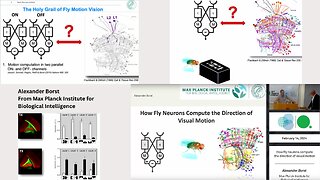
2 months agoAlexander Borst - Max Planck Institute for Biological Intelligence Presents Visuals Motion in Fly
42 -
![[Full Audiobook] Prollu: The Play](https://hugh.cdn.rumble.cloud/s/s8/1/Q/_/k/c/Q_kcp.0kob-small-Full-Audiobook-Prollu-The-P.jpg) 52:11
52:11
Prince Tanaka XI
5 months ago[Full Audiobook] Prollu: The Play
15 -
 1:01:24
nonvaxer420
1 month agoCan Mathematics Understand the Brain? - Prof. Alain Goriely, Oxford 2017
2.3K1 -
 39:35
39:35
TheMostHatedResearcher2030IoBnT
4 months agoHDIAC Podcast - Weaponizing Brain Science: Neuroweapons
44